Performance Tuning Queries in PostgreSQL

Database performance tuning: developers usually either love it or loathe it. I happen to be one that enjoys it and want to share some of the techniques I’ve been using lately to tune poor performing queries in PostgreSQL. This is not meant to be exhaustive but more of a primer for those just getting their feet wet with tuning.

Finding Slow Queries

One obvious way to start with tuning is to find specific statements that are performing poorly.

pg_stats_statements

The pg_stats_statements module is a great place to start. It simply tracks execution statistics of SQL statements and can be an easy way to find poor performing queries.

Once you have this module installed, a system view named pg_stat_statements will be available with all sorts of goodness. Once it has had a chance to collect a good amount of data, look for queries that have relatively high total_time value. Focus on these statements first.

SELECT *
FROM
  pg_stat_statements
ORDER BY
  total_time DESC;

user_id	dbid	queryid	query	calls	total_time
16384	16385	2948	SELECT address_1 FROM addresses a INNER JOIN people p ON a.person_id = p.id WHERE a.state = @state_abbrev;	39483	15224.670
16384	16385	924	SELECT person_id FROM people WHERE name = @name;	26483	12225.670
16384	16385	395	SELECT _ FROM orders WHERE EXISTS (select _ from products where is_featured = true)	18583	224.67

auto_explain

The auto_explain module is also helpful for finding slow queries but has 2 distinct advantages: it logs the actual execution plan and supports logging nested statements using the log_nested_statements option. Nested statements are those statements that are executed inside a function. If your application uses many functions, auto_explain is invaluable for getting detailed execution plans.

The log_min_duration option controls which query execution plans are logged, based on how long they perform. For example, if you set this to 1000, all statements that run longer than 1 second will be logged.

Index Tuning

Another important tuning strategy is to ensure indexes are being properly used. As a prerequisite, we need to turn on the Statistics Collector.

The Postgres Statistics Collector is a first class subsystem that collects all sorts of performance statistics that are useful.

Turning this collector on gives you tons of pg_stat_... views which contain all the goodness. In particular, I have found it to be particularly useful for finding missing and unused indexes.

Missing Indexes

Missing indexes can be one of the easiest solutions to increasing query performance. However, they are not a silver bullet and should be used properly (more on that later). If you have The Statistics Collector turned on, you can run the following query (source).

SELECT
  relname,
  seq_scan - idx_scan AS too_much_seq,
  CASE
    WHEN
      seq_scan - coalesce(idx_scan, 0) > 0
    THEN
      'Missing Index?'
    ELSE
      'OK'
  END,
  pg_relation_size(relname::regclass) AS rel_size, seq_scan, idx_scan
FROM
  pg_stat_all_tables
WHERE
  schemaname = 'public'
  AND pg_relation_size(relname::regclass) > 80000
ORDER BY
  too_much_seq DESC;

This finds tables that have had more Sequential Scans than Index Scans, a telltale sign that an index will usually help. This isn’t going to tell you which columns to create the index on so that will require a bit more work. However, knowing which table(s) need them is a good first step.

Unused Indexes

Index all the things right? Did you know having unused indexes can negatively affect write performance? The reason is, when you create an index, Postgres is burdened with the task of keeping this index updated after write (INSERT / UPDATE / DELETE) operations. So, adding an index is a balancing act because they can speed up reading of data (if created properly) but will slow down write operations. To find unused indexes you can run the following command.

SELECT
  indexrelid::regclass as index,
  relid::regclass as table,
  'DROP INDEX ' || indexrelid::regclass || ';' as drop_statement
FROM
  pg_stat_user_indexes
  JOIN
    pg_index USING (indexrelid)
WHERE
  idx_scan = 0
  AND indisunique is false;

A note about statistics on development environments

Relying upon statistics generated from a local development database can be problematic. Ideally you are able to pull the above statistics from your production machine or generate them from a restored production backup. Why? Environmental factors can and do change the way Postgres query optimizer works. Two examples:

when a machine has less memory PostgreSQL may not be able to perform a Hash Join when otherwise it would be able to and would make the join faster.
if there are not many rows in a table (like in a development database), PostgresSQL may chose to do Sequential Scans on a table rather than utilize an available index. When table sizes are small, a Seq Scan can be faster. (Note: you can run SET enable_seqscan = OFF; in a session to get the optimizer to prefer using indexes even when a Sequential Scan may be faster. This is useful when working with development databases that do not have much data in them)

Understanding Execution Plans

Now that you’ve found some statements that are slow, it’s time for the fun to begin.

EXPLAIN

The EXPLAIN command is by far the must have when it comes to tuning queries. It tells you what is really going on. To use it, simply prepend your statement with EXPLAIN and run it. PostgreSQL will show you the execution plan it used.

When using EXPLAIN for tuning, I recommend always using the ANALYZE option (EXPLAIN ANALYZE) as it gives you more accurate results. The ANALYZE option actually executes the statement (rather than just estimating it) and then explains it.

Let’s dive in and start understanding the output of EXPLAIN. Here’s an example:

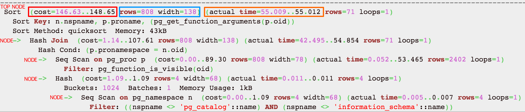
Nodes

The first thing to understand is that each indented block with a preceding “->” (along with the top line) is called a node. A node is a logical unit of work (a “step” if you will) with an associated cost and execution time. The costs and times presented at each node are cumulative and roll up all child nodes. This means that the very top line (node) shows a cumulative cost and actual time for the entire statement. This is important because you can easily drill down to determine which node(s) are the bottleneck(s).

Cost

cost=146.63..148.65

The first number is start up cost (cost to retrieve first record) and the second number is the cost incurred to process entire node (total cost from start to finish).

The cost is effectively how much work PostgreSQL estimates it will have to do to run the statement. This number is not how much time is required, although there is usually direct correlation to time required for execution. Cost is a combination of 5 work components used to estimate the work required: sequential fetch, non-sequential (random) fetch, processing of row, processing operator (function), and processing index entry. The cost represents I/O and CPU activity and the important thing to know here is that a relatively higher cost means PostgresSQL thinks it will have to do more work. The optimizer makes its decision on which execution plan to use based on the the cost. Lower costs are preferred by the optimizer.

Actual time

actual time=55.009..55.012

In milliseconds, the first number is start up time (time to retrieve first record) and the second number is the time taken to process entire node (total time from start to finish). Easy to understand right?

In the example above, it took 55.009ms to get first record and 55.012ms to finish the entire node.

Learning More about Execution Plans

There are some really great articles on understanding the output of EXPLAIN and rather than attempt to rehash them here, I recommend you invest the time to really understand them more by navigating to these 2 great resources:

Query Tuning

Now that you know which statements are performing poorly and able see their execution plans, it is time to start tweaking the query to get better performance. This is where you make changes to the queries and/or add indexes to try and get a better execution plan. Start with the bottlenecks and see if there are changes you can make that reduce costs and/or execution times.

A note about data cache and comparing apples to apples

As you make changes and evaluate the resulting execution plans to see if it is better, it is important to know that subsequent executions might be relying upon data caching that yield the perception of better results. If you run a query once, make a tweak and run it a second time, it is likely it will run much faster even if the execution plan is not more favorable. This is because PostgreSQL might have cached data used in the first run and is able to use it in the second run. Therefore, you should run queries at least 3 times and average the results to compare apples to apples.

Things I’ve learned that may help get better execution plans:

Indexes
- Eliminate Sequential Scans (Seq Scan) by adding indexes (unless table size is small)
- If using a multicolumn index, make sure you pay attention to order in which you define the included columns – More info
- Try to use indexes that are highly selective on commonly-used data. This will make their use more efficient.
WHERE clause
- Avoid LIKE
- Avoid function calls in WHERE clause
- Avoid large IN() statements
JOINs
- When joining tables, try to use a simple equality statement in the ON clause (i.e. a.id = b.person_id). Doing so allows more efficient join techniques to be used (i.e. Hash Join rather than Nested Loop Join)
- Convert subqueries to JOIN statements when possible as this usually allows the optimizer to understand the intent and possibly chose a better plan
- Use JOINs properly: Are you using GROUP BY or DISTINCT just because you are getting duplicate results? This usually indicates improper JOIN usage and may result in a higher costs
- If the execution plan is using a Hash Join it can be very slow if table size estimates are wrong. Therefore, make sure your table statistics are accurate by reviewing your vacuuming strategy
- Avoid correlated subqueries where possible; they can significantly increase query cost
- Use EXISTS when checking for existence of rows based on criterion because it “short-circuits” (stops processing when it finds at least one match)
General guidelines
- Do more with less; CPU is faster than I/O
- Utilize Common Table Expressions and temporary tables when you need to run chained queries
- Avoid LOOP statements and prefer SET operations
- Avoid COUNT(*) as PostgresSQL does table scans for this (versions <= 9.1 only)
- Avoid ORDER BY, DISTINCT, GROUP BY, UNION when possible because these cause high startup costs
- Look for a large variance between estimated rows and actual rows in the EXPLAIN statement. If the count is very different, the table statistics could be outdated and PostgreSQL is estimating cost using inaccurate statistics. For example: Limit (cost=282.37..302.01 rows=93 width=22) (actual time=34.35..49.59 rows=2203 loops=1). The estimated row count was 93 and the actual was 2,203. Therefore, it is likely making a bad plan decision. You should review your vacuuming strategy and ensure ANALYZE is being run frequently enough.

credit: https://www.geekytidbits.com/performance-tuning-postgres/