the partitioning of 1TB of data on a live system, with zero downtime

Summary

A few months ago we faced an engineering challenge of having to partition a Postgres table of more than 350M rows and about 1TB in size, as we were already facing performance issues and we were expecting to triple the number of records within the next few months.

In this blog post, we will share our experience on how we tackled the problem of live table partitioning. Our objectives were: no downtime, data integrity, minimize incoming request failures and optimize the extra storage required for the operation.

Creating a partitioned table structure itself is not complicated. However, the migration of an unpartitioned table to a partitioned one on a live system with zero downtime can be challenging, and we found that online resources were not complete and always helpful to guide someone through this process. This is the reason we decided to share our experience. While there is no silver bullet, we really hope this will help others in their partitioning journey.

Jump directly to the final solution

A bit of context

The table in question had more than 350M rows at the time, and we were expecting to triple the number of records after merging an external dataset. As a result its size would increase from about 1TB to almost 2.5TB.

Table schema is the following:

  column_name          |  data_type
-----------------------+----------------------------
  id                   |  integer
  uid                  |  character varying
  type                 |  character varying
  payload              |  jsonb
  payload_hash         |  character varying
  created_at           |  timestamp 
  updated_at           |  timestamp

It is a good practice to partition such big tables not only to optimize query performance but also maintenance operations (vacuum, indexing, backups). One could start adjusting cluster-wide or table specific settings (autovacuum, analyze, etc) but even then, these processes would still need to parse a gigantic dataset when triggered leading to degraded performance for a production system. We could vertically scale in hardware but this approach not only is not cost efficient but also expedites how quickly we will hit the upper limit.

While doing research on how others tackled similar problems, we mostly came up with solutions for partitioning tables with time series data, a much easier problem to tackle but unfortunately not applicable in our use case, and a few solutions that proposed using a duplicate table which, as we are going to discuss later, did not meet our requirements of live partitioning while ensuring data integrity.

In the rest of the article we will discuss:

Partitioning strategies
Data migration approaches we investigated
Fine tuning Postgres infrastructure to support this operation
How we partitioned a table with zero downtime

Partitioning strategies

Partitioning (splitting a large table to smaller ones while maintaining at a logical level a single table) is a widely used practice to improve database performance across different areas, from query performance to maintenance operations. There are multiple articles out there that discuss in detail the benefits of partitioning, and one can read the official documentation that provides a good overall summary along with the available partitioning strategies, i.e. Range, List and Hash partitioning.

When deciding to partition a table, it is really important to design carefully how the data are going to be split or you may end up having performance issues. The idea is to cluster data that are usually accessed together in the same partition, so that most queries retrieve data from as few partitions as possible.

In our case the vast majority of the queries are based on uid that is a randomized field with infinite range.

Range partitioning

The table is partitioned into “ranges’’ defined by a key column or set of columns, with no overlap between the ranges of values assigned to different partitions. This partitioning is perfect for time series data, but not so much for our use case since the range partition requires both minimum and maximum values of the range to be specified, in order for the partition to hold values within a range provided on the partition key, or it assumes a monotonicity in the values (e.g. timeseries) so new partitioning are created when the last one approaches exhaustion.

List partitioning

The table is partitioned by explicitly listing which value(s) of the partition key appear in each partition.

This method is the perfect candidate for partitioning on a column with a predefined set of values. One has to keep an eye out because this may lead to uneven distribution of data which of course may be a good compromise depending on the data accessing patterns. For example we could have used the type column but given our query patterns this would increase the DB overhead instead of reducing it.

We tried to do a list partitioning based on the first character of the uid. This had the advantage that we could predict the partition a record lives in. However, partitioning with list is using the IN operator to match the values for each partition, which evaluates to TRUE if the operand is equal to one of a list of expressions. Unfortunately wildcards cannot be used with IN; we would need the LIKE operator which sadly is not supported in list partitioning.

Hash partitioning

Hash partitioning is similar to list partitioning, but instead of using a natural finite domain defined by the possible values of a column, it maps all possible values of a column to a finite list of possible values. The randomization used in hashing also ensures that partitions are of comparable sizes.

We decided to go with this partitioning strategy, as it definitely matches our needs to have all rows for a specific uid in the same partition and allows us to choose the number of partitions based on the total size of the partitioned table.

Data migration Strategies

Having decided on the partition strategy, we needed to find a way to migrate all the data from the unpartitioned table, to the partitioned one.

According to Postgres documentation, the fastest method for inserting a large amount of data in a table is to:

Create the table
Bulk load the table’s data using COPY
Create any indexes needed for the table

COPY is almost always faster as it will load all the rows in one command instead of using a series of INSERT commands, and creating an index on pre-existing data is quicker than updating it incrementally as each row is loaded.

However, considering the size of the dataset and the fact that we couldn’t afford any downtime for our systems, we couldn’t use the COPY for two reasons:

COPY is carried out in a single transaction; any failures during the process would cause the whole COPY to fail and we would need to start over.
Even if we managed to minimize or even eliminate the possibility for errors, we wouldn’t be able to ensure data parity between the tables as there might have been values that had changed in between the processes to export the data from the old table and import them to the new one.

Data integrity was crucial and we didn’t mind the migration process taking longer to finish, so we started exploring other possibilities.

Duplicate table

Our initial approach was to create the partitioned table and add after update triggers to the old table that would execute the same commands in the partitioned one. As a result all actions done in the old table would be also executed in the new one. We would then execute a background task to copy all data from the old to the new table. When this task was finished, we could stop using the old table and send all queries to the partitioned one.

Even though this scenario seemed easy to implement, we found issues that couldn’t be resolved:

We would need to copy all rows from the old table to the new one and there was no solid way to check data parity between the two tables, when INSERT (with ON CONFLICT statement), UPDATE and DELETE statements are issued in the old one.
Our live system does about 50K insertions/day. If a vacuum/analyze runs in parallel with data copy for any table, performance issues would arise in the live system. We could temporarily disable vacuum maintenance while the operation was running but that would lead to the following issue.
We would need to increase the storage for more than double the size of the table, since we were going to duplicate the data. Moreover, with vacuum disabled, we would also need double the storage for all the UPDATE statements (UPDATE writes a new row version for every row). In DBaaS solutions, storage reduction is a complicated operation that can rarely happen with no downtime.

View with UNION

After deciding that a duplicate table was not an option, we tried to find a way to have both tables on the live system and move data from the old table to the partitioned one in the background. When the old table was empty we would know that the migration was over.

In order to achieve that we would create a view with UNION, to return results from both tables for SELECT statements. New records will be stored in the partitioned table, and a worker will gradually move all the records from the old table to the partitioned one.

The general idea was the following:

Create the parent table, partitions and indexes
Rename the old table and create a view instead (with the same name as the old table), to combine the results from both tables
Create the necessary function and triggers to handle INSERT, UPDATE and DELETE statements for future data
Migrate the data from the old table to the partitioned one
Delete the view and rename the partitioned table to the same name as the view (and the old table before that)
Delete the old table

This approach also had some drawbacks but, generally speaking, they were less critical:

Our view was not updatable
In order for a view to be updatable, its definition must not contain set operations at the top level; UNION is one of them. To address the issue we introduced:

a function that would handle INSERT, UPDATE and DELETE statements accordingly:
INSERT: Insert values to the partitioned table
UPDATE: Check if data exists in the old table, delete them, and insert the values to the new table
DELETE: Delete rows from both tables
a trigger to execute the above function on each of the statements

INSERT queries in our codebase contain an ON CONFLICT statement

INSERT INTO sources (uid,...)
    VALUES (...)
ON CONFLICT (uid, type, payload_hash)
    DO UPDATE SET
        payload = EXCLUDED.payload

This produced the following error, when a query was handled by the view:

SQL Error [42P10]: ERROR: there is no unique or exclusion constraint matching the ON CONFLICT specification

A view cannot have any constraints, so such requests could not be handled. The solution was to disable the ON CONFLICT statement in our codebase and let the SQL function do all the handling. After the migration was finished, we would revert the changes in the code.

Disable VACUUM

We still needed to disable VACUUM operations for the duration of the process, which would result in DB bloating. However, compared to the duplicate table approach, the data lived only once in one of the two tables so UPDATE operations would happen in only one of the tables. If disabling VACUUM for the whole duration was not acceptable, we could :

Stop the background worker
VACUUM both tables
Restart the worker

This was the perfect solution for all of our needs, as it did not require any downtime and was really easy to check for parity because when the migration process was finished the old table would be empty.

Data migration plan

We had everything in place and our strategy for moving all the rows from one table to another, in batches of 100k (mainly due to memory constraints), was to run:

INSERT INTO sources
SELECT
    *
FROM
    sources_old
LIMIT 100000;

With a function and triggers to handle INSERT, UPDATE and DELETE statements, this would essentially:

Select the rows from the old table
Try to insert the values in the view
The trigger would capture the INSERT statement and execute a function
The function would execute code depending on the event the trigger was called for

There was one particular issue with this query: It didn’t use any indexes and Postgres would perform a sequential scan on the table, which would be time consuming.

PostgreSQL automatically creates a unique index when a unique constraint or primary key is defined for a table, and since the primary key of the table is defined as SERIAL (used to generate a sequence of auto-incrementing integers), we updated the query as follows:

INSERT INTO sources
SELECT
    *
FROM
    sources_old
WHERE
    id BETWEEN <FIRST_VAL> AND <LAST_VAL>;

The plan was to get the min and max id values and process the values in between, in ranges.

Challenges

Fighting with AWS Hardware

Our database is running on RDS. RDS makes it easy to set up, operate, and scale a relational database but under the hood it uses a combination of different, interconnected services: EC2 and EBS. EC2 provides scalable computing capacity while EBS provides block level storage volumes. We are using a db.m5.large instance with a general purpose storage volume. Great for keeping the system running with no issues while keeping the cost at a minimum, and serving moderate traffic with a few spikes every now and then. However, using cloud services comes with many moving parts you need to take into account when designing a system, and RDS is no exception.

Especially in AWS, hardware comes bundled together, you cannot fine tune it to your liking to get some extra CPU, or memory, or network performance, but you will probably need to choose between predefined tiers instead. Apart from the predefined combinations of resources you need to get to the specifics of each tier regarding EBS performance, to understand how it will behave and what is expected. As we describe in this section, it gets very tricky to compute the expected performance, identify bottlenecks and figure out how to overcome them.

In order to get an estimate on performance and duration of the operation we followed these steps:

Get a fork of the database
Migrate a few 100k batches
Use the rule of three to get an estimate for the entire dataset.

Our original estimate was that the operation needed ~32h to complete. This was very misleading because the storage supports burstable performance, so for a short period of time we could reach a high performance level but this would not be sustainable. After a few more tests our estimate was corrected to ~7d, and that was on an isolated instance with no production traffic. Looking at the metrics it was clear we were IO bound.

You would think, easy just switch to a provisioned IOPS disk to ensure predictable and sustainable IO performance. Not really…

The vast majority of RDS tiers are EBS optimized, meaning they have dedicated throughput to their storage so that network traffic to the instance and the EBS volume are kept separate. However, small, medium and some of the large tiers do not sustain the maximum performance with their volumes indefinitely; they can support maximum performance for 30 minutes at least once every 24 hours, after which they revert to their baseline performance. We needed to reverse engineer the behavior so that we could figure out what hardware type we should use to achieve the throughput we needed.

According to AWS EBS throughput is calculated using the following equation:

Throughput = Number of IOPS * size per I/O operation

Each of these factors affects the others, and different workloads are more sensitive to one factor or another. Our instance could get a burst throughput to ~600MB/sec and our disk could go as high as ~8k IOPS.

Apart from provisioned IOPS for the disk, we also needed hardware that could sustain the maximum performance indefinitely throughout the whole operation. Such an instance came with more than enough resources in terms of memory and CPU, so we increased the batch-size and sped up things even more. We upgraded the instance to db.r5.4xlarge as it was the first tier in the list with consistent EBS performance, and a disk with 12k IOPS. Anything less than that would not allow us to scale high in terms of throughput.

When we rerun the isolated test, the estimate went down again to ~32h 🎉 The good news was that we had managed to sustain a certain level of performance but we noticed that a single process would cause an average of ~5k IOPS. It was unclear what the bottleneck was, but optimal performance depends on many factors, i.e. sequential vs non-sequential reads/writes, size per I/O operation, the time each operation takes to complete, the kernel of the underlying OS, and so forth and so on.

At that point nothing made sense. Although we spent some time trying to figure out the issue, with the help of dedicated guides from AWS on performance tips and instructions on how to benchmark EBS volumes, we needed to move forward due to time constraints. At this point we decided to take a leap of faith and see if parallelization could improve our results so we rerun the tests with 2 parallel migration processes. The result was what we thought it would be: twice the IOPS and throughput. We let our test run for 12h to see if performance would be consistent, and it was.

We repeated the test with 4 processes and noticed that we had better performance and throughput, and that we had managed to achieve the desired consistency in both.

To summarize the final hardware setup we used for this operation:

Instance: db.m5.large -> db.r5.4xlarge (smallest tier with guaranteed EBS performance)
Storage: 2TB gp2 -> 2TB with 20k provisioned IOPs
Workers: 4 parallel migration processes

Migration worker

Having a migration plan in place we needed to write a worker that would implement all the business logic. As mentioned earlier, our plan was to get the min(id) and max(id) values and migrate all rows in between, in batches. The worker would get the id values, split them in equal parts and parallelize the migration across multiple processes. Each process would be assigned with a list of ids, and would migrate them in batches until it was finished.

Having decided to go with 4 parallel processes for migrating the data, we needed to ensure that each process would migrate a unique range of values in order to avoid conflicts with transactions, waiting for one another. As we were about to perform the migration on a live system, we did expect such conflicts between the migration processes and the application, but these would happen occasionally (if at all) and those were the exceptions we needed to handle.

In addition to the above we had to keep a state in order to be able to stop if something went wrong, and resume from where we left off. We decided that, since this would be a one-off process, running the migration worker in a VM in the same network as our database, and using the filesystem to read/write any data was a better option, as opposed to running the worker in a container and using another database for state persistence.

For creating unique ranges of ids for each process, we exported the entire list of values and split it into 4, equally sized lists (of 140M values each). Each process would parse its assigned list, migrating all the values BETWEEN the first and the 1 millionth id in the list, in a single transaction. Upon finishing successfully, the ids would be deleted from the list and the process would continue with the next batch.

How we migrated with zero downtime

This section describes the exact actions we did, along with the corresponding SQL statements, in order to perform the migration of data to the partitioned table, with no downtime.

Prepare the database

The definition of the unpartitioned table was the following:

CREATE TABLE IF NOT EXISTS sources (
    id bigserial NOT NULL,
    uid varchar(255) NOT NULL,
    TYPE VARCHAR(50) NOT NULL,
    payload jsonb NOT NULL,
    payload_hash varchar(32) NOT NULL,
    created_at timestamp NOT NULL,
    updated_at timestamp NOT NULL,
    CONSTRAINT duplicate_sources UNIQUE (uid, TYPE, payload_hash),
    CONSTRAINT sources_pkey PRIMARY KEY (id))

We created the partitioned table with the exact same definition but with a different primary key because the partition key must be part of the primary key.

CREATE TABLE IF NOT EXISTS sources_partitioned (
    id bigserial NOT NULL,
    uid varchar(255) NOT NULL,
    TYPE VARCHAR(50) NOT NULL,
    payload jsonb NOT NULL,
    payload_hash varchar(32) NOT NULL,
    created_at timestamp NOT NULL,
    updated_at timestamp NOT NULL,
    CONSTRAINT duplicate_sources_partitioned UNIQUE (uid, TYPE, payload_hash),
    CONSTRAINT sources_partitioned_pkey PRIMARY KEY (id, uid)
)
PARTITION BY HASH (uid);

After that we created the corresponding partitions. The number of partitions will differ in each case, but in ours, and as we expect a table size of about 2TB of data, we decided to create 20 partitions of 100GB each:

CREATE TABLE sources_partition_00 PARTITION OF sources_partitioned
FOR VALUES WITH (MODULUS 20, REMAINDER 0);

CREATE TABLE sources_partition_01 PARTITION OF sources_partitioned
FOR VALUES WITH (MODULUS 20, REMAINDER 1);
-- ...
CREATE TABLE sources_partition_20 PARTITION OF sources_partitioned
FOR VALUES WITH (MODULUS 20, REMAINDER 19);

Then we created the required triggers for each of the table partitions, for the updated_at column:

CREATE TRIGGER insert_to_updated_at_sources_partition
    BEFORE UPDATE ON public.sources_partition_00
    FOR EACH ROW
    EXECUTE FUNCTION update_updated_at_column ();

CREATE TRIGGER insert_to_updated_at_sources_partition
    BEFORE UPDATE ON public.sources_partition_01
    FOR EACH ROW
    EXECUTE FUNCTION update_updated_at_column ();
-- ...
CREATE TRIGGER insert_to_updated_at_sources_partition
    BEFORE UPDATE ON public.sources_partition_19
    FOR EACH ROW
    EXECUTE FUNCTION update_updated_at_column ();

A really tricky part was the auto-increment id. We wanted to keep the original because we use them for ordering. As a result, the insertions in the partitioned table should start after the max id of the existing table. In order to do that we changed the id sequence value:

SELECT
    setval('sources_partitioned_id_seq', (
            SELECT
                MAX(id)
            FROM sources) + 1000);

+ 1000 was a safety precaution because the migration would run on a live system which may have running insertions, so we needed a buffer to make sure that ids will not overlap. That value was calculated based on the insertion rate per minute.

After that we disabled autovacuum in the old table and renamed it, so that we could create a view with the same name:

ALTER TABLE sources SET (autovacuum_enabled = FALSE, toast.autovacuum_enabled = FALSE);
ALTER TABLE sources RENAME TO sources_old;

CREATE OR REPLACE VIEW sources AS
SELECT
    *
FROM
    sources_old
UNION ALL
SELECT
    *
FROM
    sources_partitioned;

Next we created the trigger function:

CREATE OR REPLACE FUNCTION move_to_partitioned ()
    RETURNS TRIGGER
    LANGUAGE plpgsql
    AS $
    TRIG
$ DECLARE old_id bigint;
old_created timestamp;
BEGIN
    IF TG_OP = 'INSERT' THEN
        DELETE FROM sources_old ps
        WHERE ps.uid = NEW.uid
            AND ps.type = NEW.type
            AND ps.payload_hash = NEW.payload_hash
        RETURNING
            id,
            created_at INTO old_id,
            old_created;
IF FOUND THEN
    INSERT INTO sources_partitioned (id, uid, history_duplicate_ids, TYPE, payload, payload_hash, created_at, updated_at)
        VALUES (old_id, NEW.uid, NEW.history_duplicate_ids, NEW.type, NEW.payload, NEW.payload_hash, old_created, NOW())
    ON CONFLICT (uid, TYPE, payload_hash)
        DO UPDATE SET
            payload = EXCLUDED.payload;
ELSE
    INSERT INTO sources_partitioned (uid, history_duplicate_ids, TYPE, payload, payload_hash, created_at, updated_at)
        VALUES (NEW.uid, NEW.history_duplicate_ids, NEW.type, NEW.payload, NEW.payload_hash, NOW(), NOW())
    ON CONFLICT (uid, TYPE, payload_hash)
        DO UPDATE SET
            payload = EXCLUDED.payload;
END IF;
RETURN NEW;
ELSIF TG_OP = 'DELETE' THEN
    DELETE FROM sources_partitioned
    WHERE id = OLD.id;
DELETE FROM sources_old
WHERE id = OLD.id;
RETURN OLD;
ELSIF TG_OP = 'UPDATE' THEN
    DELETE FROM sources_old
    WHERE id = OLD.id;
IF FOUND THEN
    INSERT INTO sources_partitioned (id, uid, history_duplicate_ids, TYPE, payload, payload_hash, created_at, updated_at)
        VALUES (OLD.id, NEW.uid, NEW.history_duplicate_ids, NEW.type, NEW.payload, NEW.payload_hash, OLD.created_at, OLD.updated_at)
    ON CONFLICT (uid, TYPE, payload_hash)
        DO UPDATE SET
            payload = EXCLUDED.payload;
END IF;
RETURN NEW;
END IF;
END $ TRIG $;

Finally we defined when the trigger is applied to the view:

CREATE TRIGGER view_trigger
    INSTEAD OF INSERT OR UPDATE OR DELETE ON sources
    FOR EACH ROW
    EXECUTE FUNCTION move_to_partitioned ();

Database preparation was done by the application in the form of migration scripts. Once the scripts had finished, we started the worker to migrate the data from the old table to the partitioned one.

Conclusion

The migration took 36h to finish; a result we were extremely happy with, and performance was more than acceptable for such a heavy operation. Although we’ve had a few mishaps it was nothing we were not prepared for (an occasional crash and restart of a migration task) and most importantly this was completely transparent to our users since the application continued to serve traffic throughout this operation with slightly degraded performance.

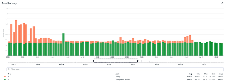
We managed to maintain the same read latency from the database.

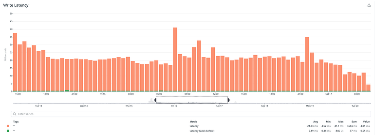
Write latency was considerably higher, which was expected due to the nature of the operation, but it stayed within acceptable limits.

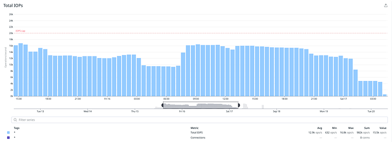
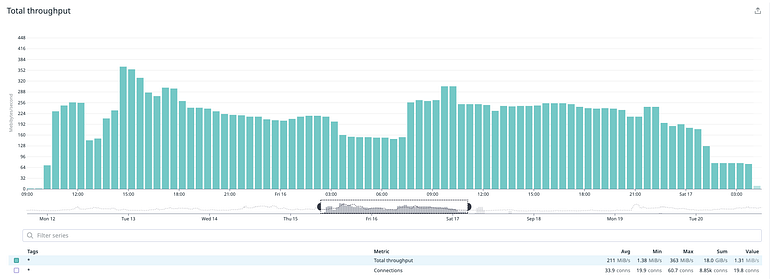
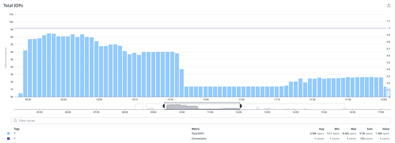
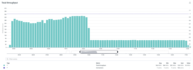
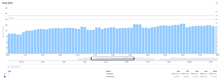
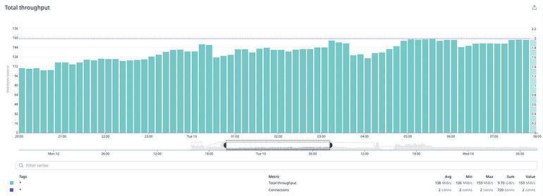
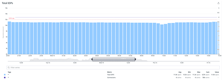
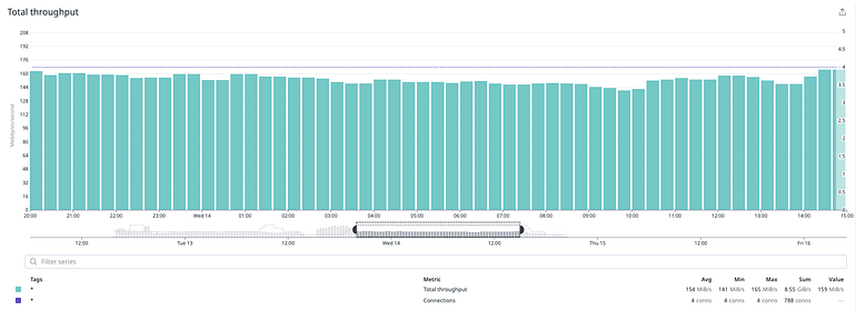
How did we do in terms of performance? For the most part we did manage to reach and sustain the expected levels of IOPS and throughput.

credit: https://engineering.workable.com/postgres-live-partitioning-of-existing-tables-15a99c16b291

DBA Notes

Postgres — Live Table Partitioning

Summary

A bit of context

Partitioning strategies

Range partitioning

List partitioning

Hash partitioning

Data migration Strategies

Duplicate table

View with UNION

Data migration plan

Challenges

Fighting with AWS Hardware

Migration worker

How we migrated with zero downtime

Prepare the database

Conclusion

Summary

A bit of context

Partitioning strategies

Range partitioning

List partitioning

Hash partitioning

Data migration Strategies

Duplicate table

View with UNION

Data migration plan

Challenges

Fighting with AWS Hardware

Migration worker

How we migrated with zero downtime

Prepare the database

Conclusion

Related posts: