When a SQL statement is sent to a PostgreSQL server for execution, Postgres will decipher various parts of the query and define an execution plan in an attempt to retrieve and manipulate that data in the most effective way possible The great news is that you can view these plans to gain insight into how your queries are interpreted, and tune them to make your queries faster than ever!

Before diving into the query plans, it will be helpful to know your tables: the number of rows stored in the table (that Postgres might have to loop through), the columns which have indexes (so an index scan can be performed as opposed to sequential scan) and the typical way of querying the data.

Examining Postgres EXPLAIN, the Holy Grail of Query Optimization

EXPLAIN [ANALYZE] statement

This command displays the execution plan that the PostgreSQL planner generates for the supplied statement. The execution plan shows how the table(s) referenced by the statement will be scanned — by plain sequential scan, index scan, etc. — and if multiple tables are referenced, what join algorithms will be used to bring together the required rows from each input table, plus any auxiliary steps needed, such as sort nodes or aggregate-function calculation nodes.

If you run EXPLAIN with ANALYZE option, the statement is not only planned but also executed. The total elapsed time expended within each plan node (in milliseconds) and total number of rows the query actually returned are added to the display. This is useful for seeing whether the planner’s estimates are close to reality.

Let’s walk through a real example

Let’s walk through a simple query involving three tables: listings, search_keys, and markets. The listings table is used to store data relevant to a listing, the search_keys table contains all the data needed for home search based on various filters, and the markets table stores information about a real estate market. The goal of the query is to find all rows in the search_keys table within a range of listing ids, which are also present in the listings table for a given market where country_code is null or US.

EXPLAIN ANALYZE
SELECT
*
From
search_keys this_
LEFT OUTER JOIN listings listing1_ on this_.listing_id = listing1_.listing_id
LEFT OUTER JOIN markets market4_ on this_.primary_market_id = market4_.market_id
WHERE
listing1_.listing_id between 113115554 and 113125553
AND (listing1_.country_code is null or listing1_.country_code='US')

The generated query plan looks like:

QUERY PLAN
--------------------------------------
Hash Left Join  (cost=7.92..6981.79 rows=12762 width=8369) (actual time=2.375..473.754 rows=30 loops=1)
Hash Cond: (this_.primary_market_id = market4_.market_id)
->  Nested Loop  (cost=0.99..6829.09 rows=12762 width=1253) (actual time=1.880..473.134 rows=30 loops=1)
->  Index Scan using listings_pkey on listings listing1_  (cost=0.57..1196.67 rows=9273 width=827) (actual time=0.685..452.927 rows=9896 loops=1)
Index Cond: ((listing_id >= '113115554'::bigint) AND (listing_id <= '113125553'::bigint))
Filter: ((country_code IS NULL) OR (country_code = 'US'::text))
Rows Removed by Filter: 104
->  Index Scan using search_keys_listing on search_keys this_  (cost=0.43..0.60 rows=1 width=426) (actual time=0.002..0.002 rows=0 loops=9896)
Index Cond: (listing_id = listing1_.listing_id)
->  Hash  (cost=5.89..5.89 rows=83 width=7116) (actual time=0.456..0.456 rows=83 loops=1)
Buckets: 1024  Batches: 1  Memory Usage: 271kB
->  Index Scan using markets_pkey on markets market4_  (cost=0.14..5.89 rows=83 width=7116) (actual time=0.003..0.176 rows=83 loops=1)
Execution time: 474.093 ms
(13 rows)

The structure of the query is

Hash Join--> Nested Loop Join    --> Index Scan on listings    --> Index Scan on search_keys--> Hash    --> Index Scan on markets

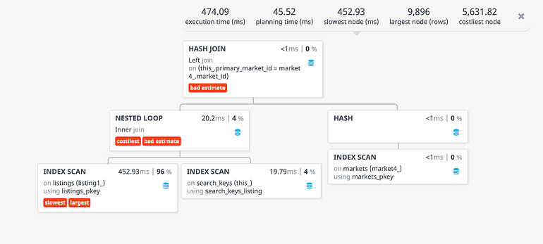
The query involves three tables and the final result is built by a tree of join steps, each with two inputs. A nested loop join is performed on listings and search_keys table, the result of which is joined with the markets table using Hash join strategy. You can also view the query plan using Postgres Explain Visualizer (pev) (shown below) or PostgreSQL’s explain analyze made readable which makes the plan easier to grok.

The visualizer needs the plan in JSON format, so you will have to run EXPLAIN with FORMAT JSON option.

Let’s dig deeper into each of these steps.

Nested Loop Join

The simplest of all join strategies, a nested loop join works by fetching the result from the left relation (listings), and for each row of the result, iterating over the right relation (search_keys) to find matching rows. Let’s look deeper at each row of nested loop join:

Nested Loop (cost=0.99..6829.09 rows=12762 width=1253) (actual time=1.880..473.134 rows=30 loops=1)

This node represents the action taken (“Nested loop”). The numbers that are quoted in the cost estimate (cost=0.99..6829.09 rows=12762 width=1253) are (left to right):

Estimated start-up cost. This is the time (ms) at which this node can begin working.
Estimated total cost. This is stated on the assumption that the plan node is run to completion, i.e., all available rows are retrieved. In practice a node’s parent node might stop short of reading all available rows (see the LIMIT example below).
Estimated number of rows output by this plan node.
Estimated average width of rows output by this plan node (in bytes).

Since we ran EXPLAIN with the ANALYZE option, the query was actually executed and timing information was captured with (actual time=1.880..473.134 rows=30 loops=1) in the plan node. The numbers depict the actual start up time (1.880 ms) when the node began execution, the total time taken for node to execute (473.134 ms), the number of rows returned by the node (30) and the number of times nested loop was executed 1 time (loops value).

In the case when a node is executed more than once, the actual time is an average of each iteration and we would multiply the value by the number of loops to get total time.

Next, let’s look at the sub actions for Nested Loop node.

Index Scan using listings_pkey on listings listing1_ (cost=0.57..1196.67 rows=9273 width=827) (actual time=0.685..452.927 rows=9896 loops=1)Index Cond: ((listing_id >= ‘113115554’::bigint) AND (listing_id <= '113125553'::bigint))Filter: ((country_code IS NULL) OR (country_code = 'US'::text))Rows Removed by Filter: 104

Postgres performs an index scan on the listings relation using listings_pkey as its scan key to fetch listing_id(s) that match the index condition. The index condition corresponds to the SQL where listing1_.listing_id between 113115554 and 113125553. The Filter condition shows the number of rows removed by filter condition (listing1_.country_code is null or listing1_.country_code='US')

Next, for each listing_id returned by the above step, postgres performs an index scan on search_keys to find matching rows.

Index Scan using search_keys_listing on search_keys this_ (cost=0.43..0.60 rows=1 width=426) (actual time=0.002..0.002 rows=0 loops=9896)Index Cond: (listing_id = listing1_.listing_id)

The loops value reports the total number of executions of the node. The actual time and rows values shown are averages per loop execution. This is done to make the numbers comparable with the way that the cost estimates are shown. To get the total time and rows, the actual time and rows value need to be multiplied by loops values. However since postgres rounds up these averages, the actual row values are shown as zero.

The result of the nested loop action is joined with the markets table using hash join strategy.

Hash Join

This join strategy involves scanning the right relation first and loading it into a hash table, using its join attributes as hash keys. Next the left relation is scanned and the appropriate values of every row found are used as hash keys to locate the matching rows in the hash table.

Hash Left Join (cost=7.92..6981.79 rows=12762 width=8369) (actual time=2.375..473.754 rows=30 loops=1)Hash Cond: (this_.primary_market_id = market4_.market_id)

The above node represents the estimated and actual cost of hash join of the result of nested loop join and markets.

Let’s look into the node which loads the markets relation to a hash table using market_id as its hash key.

Hash (cost=5.89..5.89 rows=83 width=7116) (actual time=0.456..0.456 rows=83 loops=1)Buckets: 1024 Batches: 1 Memory Usage: 271kB-> Index Scan using markets_pkey on markets market4_ (cost=0.14..5.89 rows=83 width=7116) (actual time=0.003..0.176 rows=83 loops=1)

The Hash node includes information about the number of hash buckets and batches, as well as peak memory usage along with estimated and actual costs of building up the hash table.

After the hash table is built, the result of the nested loop join is scanned and using the primary_market_id as the hash key the hash table is probed to find all matching rows. (Hash Condition in hash join node).

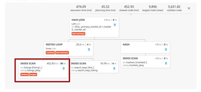
Can we optimize the query?

In the query plan, the majority of the time (452.93 ms out of total 474.09 ms) is spent in the index scan of listings table to find the range between 113115554 and 113125553 which returns 9896 rows.

The corresponding query plan row is:

Index Scan using listings_pkey on listings listing1_ (cost=0.57..1196.67 rows=9273 width=827) (actual time=0.685..452.927 rows=9896 loops=1)

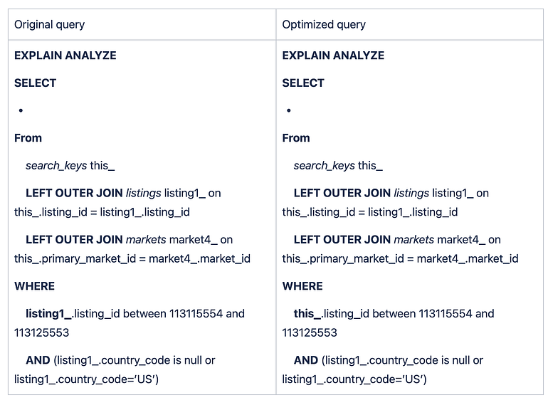
You will notice that the final result of the nested loop join between listings and search_keys table returns only 30 rows out of 9896 rows matched from the listings table. Looking closely, the listings and search_keys tables are joined on the listing table’s id, which has a far higher number of matching rows for the range of listing ids than what is needed.

Let’s modify the query’s WHERE clause to select listing ids in desired range from search_keys table instead of listings.

The execution plan for above query is:

QUERY PLAN
-----------------------------------
Hash Left Join  (cost=7.92..303.55 rows=303 width=8369) (actual time=1.138..12.669 rows=30 loops=1)
Hash Cond: (this_.primary_market_id = market4_.market_id)
->  Nested Loop Left Join  (cost=0.99..293.17 rows=303 width=1253) (actual time=0.501..11.987 rows=30 loops=1)
Filter: ((listing1_.country_code IS NULL) OR (listing1_.country_code = 'US'::text))
Rows Removed by Filter: 7
->  Index Scan using search_keys_listing on search_keys this_  (cost=0.43..38.76 rows=319 width=426) (actual time=0.050..5.378 rows=37 loops=1)
Index Cond: ((listing_id >= '113115554'::bigint) AND (listing_id <= '113125553'::bigint))
->  Index Scan using listing_id_available_photos on listings listing1_  (cost=0.57..0.79 rows=1 width=827) (actual time=0.175..0.175 rows=1 loops=37)
Index Cond: (this_.listing_id = listing_id)
->  Hash  (cost=5.89..5.89 rows=83 width=7116) (actual time=0.586..0.586 rows=83 loops=1)
Buckets: 1024  Batches: 1  Memory Usage: 271kB
->  Index Scan using markets_pkey on markets market4_  (cost=0.14..5.89 rows=83 width=7116) (actual time=0.004..0.263 rows=83 loops=1)
Execution time: 13.070 ms
(13 rows)

The optimized query takes 13 ms compared to 474 ms earlier. The key difference here is:

Index Scan using search_keys_listing on search_keys this_ (cost=0.43..38.76 rows=319 width=426) (actual time=0.050..5.378 rows=37 loops=1)Index Cond: ((listing_id >= '113115554'::bigint) AND (listing_id <= '113125553'::bigint))

An Index Scan on search_keys table is performed to find listings with ids in range ('113115554' and '113125553') which takes 5.378 ms and returns 37 rows in contrast to 9896 rows in 452.927 ms returned by the previous execution plan that scanned listings table for the same.

More Resources

https://www.postgresql.org/docs/9.6/using-explain.html

https://pganalyze.com/docs/explain

https://tatiyants.com/pev/#/plans/new

PS — The query used an example here was optimized by Ken Brush and Robert Gay during a site outage event in Feb, 2020. Thanks Ken and Robert!

credit: https://redfin.engineering/postgresql-explain-explained-4a2d5c5e0ac5

DBA Notes

PostgreSQL EXPLAIN Explained

Examining Postgres EXPLAIN, the Holy Grail of Query Optimization

Let’s walk through a real example

Nested Loop Join

Hash Join

Can we optimize the query?

More Resources

Examining Postgres EXPLAIN, the Holy Grail of Query Optimization

Let’s walk through a real example

Nested Loop Join

Hash Join

Can we optimize the query?

More Resources

Related posts: