Structure
B-tree index type, implemented as “btree” access method, is suitable for data that can be sorted. In other words, “greater”, “greater or equal”, “less”, “less or equal”, and “equal” operators must be defined for the data type.
Note that the same data can sometimes be sorted differently, which takes us back to the concept of operator family.
As always, index rows of the B-tree are packed into pages. In leaf pages, these rows contain data to be indexed (keys) and references to table rows (TIDs). In internal pages, each row references a child page of the index and contains the minimal value in this page.
B-trees have a few important traits:
- B-trees are balanced, that is, each leaf page is separated from the root by the same number of internal pages. Therefore, search for any value takes the same time.
- B-trees are multi-branched, that is, each page (usually 8 KB) contains a lot of (hundreds) TIDs. As a result, the depth of B-trees is pretty small, actually up to 4–5 for very large tables.
- Data in the index is sorted in nondecreasing order (both between pages and inside each page), and same-level pages are connected to one another by a bidirectional list. Therefore, we can get an ordered data set just by a list walk one or the other direction without returning to the root each time.
Below is a simplified example of the index on one field with integer keys.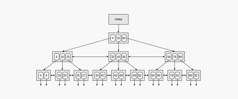
The very first page of the index is a metapage, which references the index root. Internal nodes are located below the root, and leaf pages are in the bottommost row. Down arrows represent references from leaf nodes to table rows (TIDs).
Search by equality
Let’s consider search of a value in a tree by condition “indexed-field = expression“. Say, we are interested in the key of 49.
The search starts with the root node, and we need to determine to which of the child nodes to descend. Being aware of the keys in the root node (4, 32, 64), we therefore figure out the value ranges in child nodes. Since 32 ≤ 49 < 64, we need to descend to the second child node. Next, the same process is recursively repeated until we reach a leaf node from which the needed TIDs can be obtained.
In reality, a number of particulars complicate this seemingly simple process. For example, an index can contain non-unique keys and there can be so many equal values that they do not fit one page. Getting back to our example, it seems that we should descend from the internal node over the reference to the value of 49. But, as clear from the figure, this way we will skip one of the “49” keys in the preceding leaf page. Therefore, once we’ve found an exactly equal key in an internal page, we have to descend one position left and then look through index rows of the underlying level from left to right in search of the sought key.
(Another complication is that during the search other processes can change the data: the tree can be rebuilt, pages can be split into two, etc. All algorithms are engineered for these concurrent operations not to interfere with one another and not to cause extra locks wherever possible. But we will avoid expanding on this.)
Search by inequality
When searching by the condition “indexed-field ≤ expression” (or “indexed-field ≥ expression“), we first find a value (if any) in the index by the equality condition “indexed-field = expression” and then walk through leaf pages in the appropriate direction to the end.
The figure illustrates this process for n ≤ 35: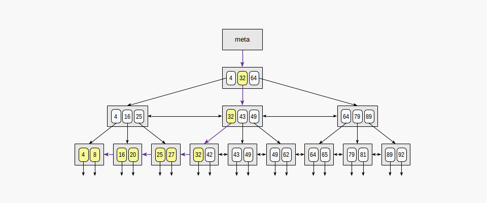
The “greater” and “less” operators are supported in a similar way, except that the value initially found must be dropped.
Search by range
When searching by range “expression1 ≤ indexed-field ≤ expression2“, we find a value by condition “indexed-field = expression1“, and then keep walking through leaf pages while the condition “indexed-field ≤ expression2” is met; or vice versa: start with the second expression and walk in an opposite direction until we reach the first expression.
The figure shows this process for condition 23 ≤ n ≤ 64: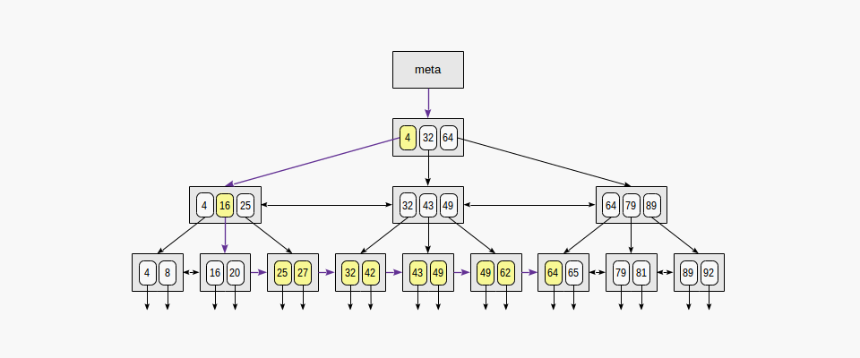
Example
Let’s look at an example of what query plans look like. As usual, we use the demo database, and this time we will consider the aircraft table. It contains as few as nine rows, and the planner would choose not to use the index since the entire table fits one page. But this table is interesting to us for an illustrative purpose.
demo=# select * from aircrafts;
 aircraft_code |        model        | range
---------------+---------------------+-------
 773           | Boeing 777-300      | 11100
 763           | Boeing 767-300      |  7900
 SU9           | Sukhoi SuperJet-100 |  3000
 320           | Airbus A320-200     |  5700
 321           | Airbus A321-200     |  5600
 319           | Airbus A319-100     |  6700
 733           | Boeing 737-300      |  4200
 CN1           | Cessna 208 Caravan  |  1200
 CR2           | Bombardier CRJ-200  |  2700
(9 rows)
demo=# create index on aircrafts(range);

demo=# set enable_seqscan = off;
(Or explicitly, “create index on aircrafts using btree(range)”, but it’s a B-tree that is built by default.)
Search by equality:
demo=# explain(costs off) select * from aircrafts where range = 3000;
                    QUERY PLAN
---------------------------------------------------
 Index Scan using aircrafts_range_idx on aircrafts
   Index Cond: (range = 3000)
(2 rows)
Search by inequality:
demo=# explain(costs off) select * from aircrafts where range < 3000;
                    QUERY PLAN
---------------------------------------------------
 Index Scan using aircrafts_range_idx on aircrafts
   Index Cond: (range < 3000)
(2 rows)
And by range:
demo=# explain(costs off) select * from aircrafts
where range between 3000 and 5000;
                     QUERY PLAN
-----------------------------------------------------
 Index Scan using aircrafts_range_idx on aircrafts
   Index Cond: ((range >= 3000) AND (range <= 5000))
(2 rows)
Sorting
Let’s once again emphasize the point that with any kind of scan (index, index-only, or bitmap), “btree” access method returns ordered data, which we can clearly see in the above figures.
Therefore, if a table has an index on the sort condition, the optimizer will consider both options: index scan of the table, which readily returns sorted data, and sequential scan of the table with subsequent sorting of the result.
Sort order
When creating an index we can explicitly specify the sort order. For example, we can create an index by flight ranges this way in particular:
demo=# create index on aircrafts(range desc);
In this case, larger values would appear in the tree on the left, while smaller values would appear on the right. Why can this be needed if we can walk through indexed values in either direction?
The purpose is multi-column indexes. Let’s create a view to show aircraft models with a conventional division into short-, middle-, and long-range craft:
demo=# create view aircrafts_v as
select model,
       case
           when range < 4000 then 1
           when range < 10000 then 2
           else 3
       end as class
from aircrafts;

demo=# select * from aircrafts_v;
        model        | class
---------------------+-------
 Boeing 777-300      |     3
 Boeing 767-300      |     2
 Sukhoi SuperJet-100 |     1
 Airbus A320-200     |     2
 Airbus A321-200     |     2
 Airbus A319-100     |     2
 Boeing 737-300      |     2
 Cessna 208 Caravan  |     1
 Bombardier CRJ-200  |     1
(9 rows)
And let’s create an index (using the expression):
demo=# create index on aircrafts(
  (case when range < 4000 then 1 when range < 10000 then 2 else 3 end),
  model);
Now we can use this index to get data sorted by both columns in ascending order:
demo=# select class, model from aircrafts_v order by class, model;
 class |        model
-------+---------------------
     1 | Bombardier CRJ-200
     1 | Cessna 208 Caravan
     1 | Sukhoi SuperJet-100
     2 | Airbus A319-100
     2 | Airbus A320-200
     2 | Airbus A321-200
     2 | Boeing 737-300
     2 | Boeing 767-300
     3 | Boeing 777-300
(9 rows)
demo=# explain(costs off)
select class, model from aircrafts_v order by class, model;
                       QUERY PLAN
--------------------------------------------------------
 Index Scan using aircrafts_case_model_idx on aircrafts
(1 row)
Similarly, we can perform the query to sort data in descending order:
demo=# select class, model from aircrafts_v order by class desc, model desc;
 class |        model
-------+---------------------
     3 | Boeing 777-300
     2 | Boeing 767-300
     2 | Boeing 737-300
     2 | Airbus A321-200
     2 | Airbus A320-200
     2 | Airbus A319-100
     1 | Sukhoi SuperJet-100
     1 | Cessna 208 Caravan
     1 | Bombardier CRJ-200
(9 rows)
demo=# explain(costs off)
select class, model from aircrafts_v order by class desc, model desc;
                           QUERY PLAN
-----------------------------------------------------------------
 Index Scan BACKWARD using aircrafts_case_model_idx on aircrafts
(1 row)
However, we cannot use this index to get data sorted by one column in descending order and by the other column in ascending order. This will require sorting separately:
demo=# explain(costs off)
select class, model from aircrafts_v order by class ASC, model DESC;
                   QUERY PLAN
-------------------------------------------------
 Sort
   Sort Key: (CASE ... END), aircrafts.model DESC
   ->  Seq Scan on aircrafts
(3 rows)
(Note that, as a last resort, the planner chose sequential scan regardless of “enable_seqscan = off” setting made earlier. This is because actually this setting does not forbid table scanning, but only sets its astronomic cost – please look at the plan with “costs on”.)
To make this query use the index, the latter must be built with the needed sort direction:
demo=# create index aircrafts_case_asc_model_desc_idx on aircrafts(
 (case
    when range < 4000 then 1
    when range < 10000 then 2
    else 3
  end) ASC,
  model DESC);

demo=# explain(costs off)
select class, model from aircrafts_v order by class ASC, model DESC;
                           QUERY PLAN
-----------------------------------------------------------------
 Index Scan using aircrafts_case_asc_model_desc_idx on aircrafts
(1 row)
Order of columns
Another issue that arises when using multi-column indexes is the order of listing columns in an index. For B-tree, this order is of huge importance: the data inside pages will be sorted by the first field, then by the second one, and so on.
We can represent the index that we built on range intervals and models in a symbolic way as follows:
Actually such a small index will for sure fit one root page. In the figure, it is deliberately distributed among several pages for clarity.
It is clear from this chart that search by predicates like “class = 3” (search only by the first field) or “class = 3 and model = ‘Boeing 777-300′” (search by both fields) will work efficiently.
However, search by the predicate “model = ‘Boeing 777-300′” will be way less efficient: starting with the root, we cannot determine to which child node to descend, therefore, we will have to descend to all of them. This does not mean that an index like this cannot ever be used – its efficiency is at issue. For example, if we had three classes of aircraft and a great many models in each class, we would have to look through about one third of the index and this might have been more efficient than the full table scan… or not.
However, if we create an index like this:
demo=# create index on aircrafts(
  model,
  (case when range < 4000 then 1 when range < 10000 then 2 else 3 end));
the order of fields will change: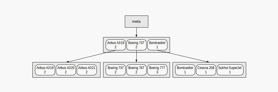
With this index, search by the predicate “model = ‘Boeing 777-300′” will work efficiently, but search by the predicate “class = 3” will not.
NULLs
“btree” access method indexes NULLs and supports search by conditions IS NULL and IS NOT NULL.
Let’s consider the table of flights, where NULLs occur:
demo=# create index on flights(actual_arrival);

demo=# explain(costs off) select * from flights where actual_arrival is null;
                      QUERY PLAN
-------------------------------------------------------
 Bitmap Heap Scan on flights
   Recheck Cond: (actual_arrival IS NULL)
   ->  Bitmap Index Scan on flights_actual_arrival_idx
         Index Cond: (actual_arrival IS NULL)
(4 rows)
NULLs are located on one or the other end of leaf nodes depending on how the index was created (NULLS FIRST or NULLS LAST). This is important if a query includes sorting: the index can be used if the SELECT command specifies the same order of NULLs in its ORDER BY clause as the order specified for the built index (NULLS FIRST or NULLS LAST).
In the following example, these orders are the same, therefore, we can use the index:
demo=# explain(costs off)
select * from flights order by actual_arrival NULLS LAST;
                       QUERY PLAN
--------------------------------------------------------
 Index Scan using flights_actual_arrival_idx on flights
(1 row)
And here these orders are different, and the optimizer chooses sequential scan with subsequent sorting:
demo=# explain(costs off)
select * from flights order by actual_arrival NULLS FIRST;
               QUERY PLAN
----------------------------------------
 Sort
   Sort Key: actual_arrival NULLS FIRST
   ->  Seq Scan on flights
(3 rows)
To use the index, it must be created with NULLs located at the beginning:
demo=# create index flights_nulls_first_idx on flights(actual_arrival NULLS FIRST);

demo=# explain(costs off)
select * from flights order by actual_arrival NULLS FIRST;
                     QUERY PLAN
-----------------------------------------------------
 Index Scan using flights_nulls_first_idx on flights
(1 row)
Issues like this are certainly caused by NULLs not being sortable, that is, the result of comparison for NULL and any other value is undefined:
demo=# \pset null NULL

demo=# select null < 42;
 ?column?
----------
 NULL
(1 row)
This runs counter to the concept of B-tree and does not fit into the general pattern. NULLs, however, play such an important role in databases that we always have to make exceptions for them.
Since NULLs can be indexed, it is possible to use an index even without any conditions imposed on the table (since the index contains information on all table rows for sure). This may make sense if the query requires data ordering and the index ensures the order needed. In this case, the planner can rather choose index access to save on separate sorting.
Properties
Let’s look at properties of “btree” access method (queries have already been provided).
 amname |     name      | pg_indexam_has_property
--------+---------------+-------------------------
 btree  | can_order     | t
 btree  | can_unique    | t
 btree  | can_multi_col | t
 btree  | can_exclude   | t
As we’ve seen, B-tree can order data and supports uniqueness – and this is the only access method to provide us with properties like these. Multicolumn indexes are also permitted, but other access methods (although not all of them) may also support such indexes. We will discuss support of EXCLUDE constraint next time, and not without reason.
     name      | pg_index_has_property
---------------+-----------------------
 clusterable   | t
 index_scan    | t
 bitmap_scan   | t
 backward_scan | t
“btree” access method supports both techniques to get values: index scan, as well as bitmap scan. And as we could see, the access method can walk through the tree both “forward” and “backward”.
        name        | pg_index_column_has_property
--------------------+------------------------------
 asc                | t
 desc               | f
 nulls_first        | f
 nulls_last         | t
 orderable          | t
 distance_orderable | f
 returnable         | t
 search_array       | t
 search_nulls       | t
First four properties of this layer explain how exactly values of a certain specific column are ordered. In this example, values are sorted in ascending order (“asc”) and NULLs are provided last (“nulls_last”). But as we’ve already seen, other combinations are possible.
“search_array” property indicates support of expressions like this by the index:
demo=# explain(costs off)
select * from aircrafts where aircraft_code in ('733','763','773');
                           QUERY PLAN
-----------------------------------------------------------------
 Index Scan using aircrafts_pkey on aircrafts
   Index Cond: (aircraft_code = ANY ('{733,763,773}'::bpchar[]))
(2 rows)
“returnable” property indicates support of index-only scan, which is reasonable since rows of the index store indexed values themselves (unlike in hash index, for example). Here it makes sense to say a few words about covering indexes based on B-tree.
Unique indexes with additional rows
As we discussed earlier, a covering index is the one that stores all values needed for a query, access to the table itself not being required (nearly). A unique index can specifically be covering.
But let’s assume that we want to add extra columns needed for a query to the unique index. Values of the new composite key may now fail to be unique, and two indexes on the same columns will then be needed: one unique (to support integrity constraint) and another one non-unique (to be used as covering). This is inefficient for sure.
In our company Anastasiya Lubennikova @lubennikovaav improved “btree” method so that additional, non-unique, columns could be included in a unique index. We hope, this patch will be adopted by the community to become a part of PostgreSQL, but this will not happen as early as in version 10. At this point, the patch is available in Pro Standard 9.5+, and this is what it looks like.
In fact this patch was committed to PostgreSQL 11.
Let’s consider the bookings table:
demo=# \d bookings
              Table "bookings.bookings"
    Column    |           Type           | Modifiers
--------------+--------------------------+-----------
 book_ref     | character(6)             | not null
 book_date    | timestamp with time zone | not null
 total_amount | numeric(10,2)            | not null
Indexes:
    "bookings_pkey" PRIMARY KEY, btree (book_ref)
Referenced by:
    TABLE "tickets" CONSTRAINT "tickets_book_ref_fkey" FOREIGN KEY (book_ref) REFERENCES bookings(book_ref)
In this table, the primary key (book_ref, booking code) is provided by a regular “btree” index. Let’s create a new unique index with an additional column:
demo=# create unique index bookings_pkey2 on bookings(book_ref) INCLUDE (book_date);
Now we replace the existing index with a new one (in the transaction, to apply all changes simultaneously):
demo=# begin;

demo=# alter table bookings drop constraint bookings_pkey cascade;

demo=# alter table bookings add primary key using index bookings_pkey2;

demo=# alter table tickets add foreign key (book_ref) references bookings (book_ref);

demo=# commit;
This is what we get:
demo=# \d bookings
              Table "bookings.bookings"
    Column    |           Type           | Modifiers
--------------+--------------------------+-----------
 book_ref     | character(6)             | not null
 book_date    | timestamp with time zone | not null
 total_amount | numeric(10,2)            | not null
Indexes:
    "bookings_pkey2" PRIMARY KEY, btree (book_ref) INCLUDE (book_date)
Referenced by:
    TABLE "tickets" CONSTRAINT "tickets_book_ref_fkey" FOREIGN KEY (book_ref) REFERENCES bookings(book_ref)
Now one and the same index works as unique and serves as a covering index for this query, for example:
demo=# explain(costs off)
select book_ref, book_date from bookings where book_ref = '059FC4';
                    QUERY PLAN
--------------------------------------------------
 Index Only Scan using bookings_pkey2 on bookings
   Index Cond: (book_ref = '059FC4'::bpchar)
(2 rows)
Creation of the index
It is well-known, yet no less important, that for a large-size table, it is better to load data there without indexes and create needed indexes later. This is not only faster, but most likely the index will have smaller size.
The thing is that creation of “btree” index uses a more efficient process than row-wise insertion of values into the tree. Roughly, all data available in the table are sorted, and leaf pages of these data are created. Then internal pages are “built over” this base until the entire pyramid converges to the root.
The speed of this process depends on the size of RAM available, which is limited by the “maintenance_work_mem” parameter. So, increasing the parameter value can speed up the process. For unique indexes, memory of size “work_mem” is allocated in addition to “maintenance_work_mem”.
Comparison semantics
Last time we’ve mentioned that PostgreSQL needs to know which hash functions to call for values of different types and that this association is stored in “hash” access method. Likewise, the system must figure out how to order values. This is needed for sortings, groupings (sometimes), merge joins, and so on. PostgreSQL does not bind itself to operator names (such as >, <, =) since users can define their own data type and give corresponding operators different names. An operator family used by “btree” access method defines operator names instead.
For example, these comparison operators are used in the “bool_ops” operator family:
postgres=# select   amop.amopopr::regoperator as opfamily_operator,
         amop.amopstrategy
from     pg_am am,
         pg_opfamily opf,
         pg_amop amop
where    opf.opfmethod = am.oid
and      amop.amopfamily = opf.oid
and      am.amname = 'btree'
and      opf.opfname = 'bool_ops'
order by amopstrategy;
  opfamily_operator  | amopstrategy
---------------------+--------------
 <(boolean,boolean)  |            1
 <=(boolean,boolean) |            2
 =(boolean,boolean)  |            3
 >=(boolean,boolean) |            4
 >(boolean,boolean)  |            5
(5 rows)
Here we can see five comparison operators, but as already mentioned, we should not rely on their names. To figure out which comparison each operator does, the strategy concept is introduced. Five strategies are defined to describe operator semantics:
- 1 — less
- 2 — less or equal
- 3 — equal
- 4 — greater or equal
- 5 — greater
Some operator families can contain several operators implementing one strategy. For example, “integer_ops” operator family contains the following operators for strategy 1:
postgres=# select   amop.amopopr::regoperator as opfamily_operator
from     pg_am am,
         pg_opfamily opf,
         pg_amop amop
where    opf.opfmethod = am.oid
and      amop.amopfamily = opf.oid
and      am.amname = 'btree'
and      opf.opfname = 'integer_ops'
and      amop.amopstrategy = 1
order by opfamily_operator;
  opfamily_operator
----------------------
 <(integer,bigint)
 <(smallint,smallint)
 <(integer,integer)
 <(bigint,bigint)
 <(bigint,integer)
 <(smallint,integer)
 <(integer,smallint)
 <(smallint,bigint)
 <(bigint,smallint)
(9 rows)
Thanks to this, the optimizer can avoid type casts when comparing values of different types contained in one operator family.
Index support for a new data type
The documentation provides an example of creation of a new data type for complex numbers and of an operator class to sort values of this type. This example uses C language, which is absolutely reasonable when the speed is critical. But nothing hinders us from using pure SQL for the same experiment in order just to try and better understand the comparison semantics.
Let’s create a new composite type with two fields: real and imaginary parts.
postgres=# create type complex as (re float, im float);
We can create a table with a field of the new type and add some values to the table:
postgres=# create table numbers(x complex);

postgres=# insert into numbers values ((0.0, 10.0)), ((1.0, 3.0)), ((1.0, 1.0));
Now a question arises: how to order complex numbers if no order relation is defined for them in the mathematical sense?
As it turns out, comparison operators are already defined for us:
postgres=# select * from numbers order by x;
   x
--------
 (0,10)
 (1,1)
 (1,3)
(3 rows)
By default, sorting is componentwise for a composite type: first fields are compared, then second fields, and so on, roughly the same way as text strings are compared character-by-character. But we can define a different order. For example, complex numbers can be treated as vectors and ordered by the modulus (length), which is computed as the square root of the sum of squares of the coordinates (the Pythagoras’ theorem). To define such an order, let’s create an auxiliary function that computes the modulus:
postgres=# create function modulus(a complex) returns float as $$
    select sqrt(a.re*a.re + a.im*a.im);
$$ immutable language sql;
Now we will systematically define functions for all the five comparison operators using this auxiliary function:
postgres=# create function complex_lt(a complex, b complex) returns boolean as $$
    select modulus(a) < modulus(b);
$$ immutable language sql;

postgres=# create function complex_le(a complex, b complex) returns boolean as $$
    select modulus(a) <= modulus(b);
$$ immutable language sql;

postgres=# create function complex_eq(a complex, b complex) returns boolean as $$
    select modulus(a) = modulus(b);
$$ immutable language sql;

postgres=# create function complex_ge(a complex, b complex) returns boolean as $$
    select modulus(a) >= modulus(b);
$$ immutable language sql;

postgres=# create function complex_gt(a complex, b complex) returns boolean as $$
    select modulus(a) > modulus(b);
$$ immutable language sql;
And we’ll create corresponding operators. To illustrate that they do not need to be called “>”, “<“, and so on, let’s give them “weird” names.
postgres=# create operator #<#(leftarg=complex, rightarg=complex, procedure=complex_lt);

postgres=# create operator #<=#(leftarg=complex, rightarg=complex, procedure=complex_le);

postgres=# create operator #=#(leftarg=complex, rightarg=complex, procedure=complex_eq);

postgres=# create operator #>=#(leftarg=complex, rightarg=complex, procedure=complex_ge);

postgres=# create operator #>#(leftarg=complex, rightarg=complex, procedure=complex_gt);
At this point, we can compare numbers:
postgres=# select (1.0,1.0)::complex #<# (1.0,3.0)::complex;
 ?column?
----------
 t
(1 row)
In addition to five operators, “btree” access method requires one more function (excessive but convenient) to be defined: it must return -1, 0, or 1 if the first value is less than, equal to, or greater than the second one. This auxiliary function is called support. Other access methods can require defining other support functions.
postgres=# create function complex_cmp(a complex, b complex) returns integer as $$
    select case when modulus(a) < modulus(b) then -1
                when modulus(a) > modulus(b) then 1
                else 0
           end;
$$ language sql;
Now we are ready to create an operator class (and same-name operator family will be created automatically):
postgres=# create operator class complex_ops
default for type complex
using btree as
    operator 1 #<#,
    operator 2 #<=#,
    operator 3 #=#,
    operator 4 #>=#,
    operator 5 #>#,
    function 1 complex_cmp(complex,complex);
Now sorting works as desired:
postgres=# select * from numbers order by x;
   x
--------
 (1,1)
 (1,3)
 (0,10)
(3 rows)
And it will certainly be supported by “btree” index.
To complete the picture, you can get support functions using this query:
postgres=# select amp.amprocnum,
       amp.amproc,
       amp.amproclefttype::regtype,
       amp.amprocrighttype::regtype
from   pg_opfamily opf,
       pg_am am,
       pg_amproc amp
where  opf.opfname = 'complex_ops'
and    opf.opfmethod = am.oid
and    am.amname = 'btree'
and    amp.amprocfamily = opf.oid;
 amprocnum |   amproc    | amproclefttype | amprocrighttype
-----------+-------------+----------------+-----------------
         1 | complex_cmp | complex        | complex
(1 row)
Internals
We can explore the internal structure of B-tree using “pageinspect” extension.
demo=# create extension pageinspect;
Index metapage:
demo=# select * from bt_metap('ticket_flights_pkey');
 magic  | version | root | level | fastroot | fastlevel
--------+---------+------+-------+----------+-----------
 340322 |       2 |  164 |     2 |      164 |         2
(1 row)
The most interesting here is the index level: the index on two columns for a table with one million rows required as few as 2 levels (not including the root).
Statistical information on block 164 (root):
demo=# select type, live_items, dead_items, avg_item_size, page_size, free_size
from bt_page_stats('ticket_flights_pkey',164);
 type | live_items | dead_items | avg_item_size | page_size | free_size
------+------------+------------+---------------+-----------+-----------
 r    |         33 |          0 |            31 |      8192 |      6984
(1 row)
And the data in the block (the “data” field, which is here sacrificed to the screen width, contains the value of the indexing key in binary representation):
demo=# select itemoffset, ctid, itemlen, left(data,56) as data
from bt_page_items('ticket_flights_pkey',164) limit 5;
 itemoffset |  ctid   | itemlen |                           data
------------+---------+---------+----------------------------------------------------------
          1 | (3,1)   |       8 |
          2 | (163,1) |      32 | 1d 30 30 30 35 34 33 32 33 30 35 37 37 31 00 00 ff 5f 00
          3 | (323,1) |      32 | 1d 30 30 30 35 34 33 32 34 32 33 36 36 32 00 00 4f 78 00
          4 | (482,1) |      32 | 1d 30 30 30 35 34 33 32 35 33 30 38 39 33 00 00 4d 1e 00
          5 | (641,1) |      32 | 1d 30 30 30 35 34 33 32 36 35 35 37 38 35 00 00 2b 09 00
(5 rows)
The first element pertains to techniques and specifies the upper bound of all elements in the block (an implementation detail that we did not discuss), while the data itself starts with the second element. It is clear that the leftmost child node is block 163, followed by block 323, and so on. They, in turn, can be explored using the same functions.
ref: https://postgrespro.com/blog/pgsql/4161516
